Module 1: Fundamentals of Machine Learning#
Machine Learning#
Machine Learning is a branch of artificial intelligence (AI) that centers on empowering computer systems to automatically learn and refine their performance over time without explicit programming instructions. The fundamental goal is to enable machines to recognize patterns, extract meaningful insights, and make predictions or decisions based on data.
What is Machine Learning About?#
Machine Learning dedicated to empowering computer systems to autonomously refine their performance without explicit programming instructions. The essence lies in enabling machines to discern patterns, derive valuable insights, and autonomously predict outcomes or make informed decisions based on data analysis. By leveraging algorithms, Machine Learning endeavors to facilitate the understanding and extraction of meaningful information from datasets, fostering the capability of machines to learn from experience and adapt their behavior or predictions over time.
At its core, Machine Learning revolves around the development and utilization of algorithms capable of perceiving patterns and leveraging these observations to make data-centric predictions or decisions. Through the process of training models on extensive datasets, Machine Learning endeavors to uncover correlations, trends, and underlying structures present within the data. This methodology allows computers to not only comprehend and analyze known examples but also to generalize from this knowledge, applying learned insights to novel, unseen data instances. The ultimate objective is to equip machines with the ability to extrapolate from past experiences, making informed conclusions and predictions when presented with unfamiliar scenarios, thereby enhancing their adaptability and problem-solving capabilities.
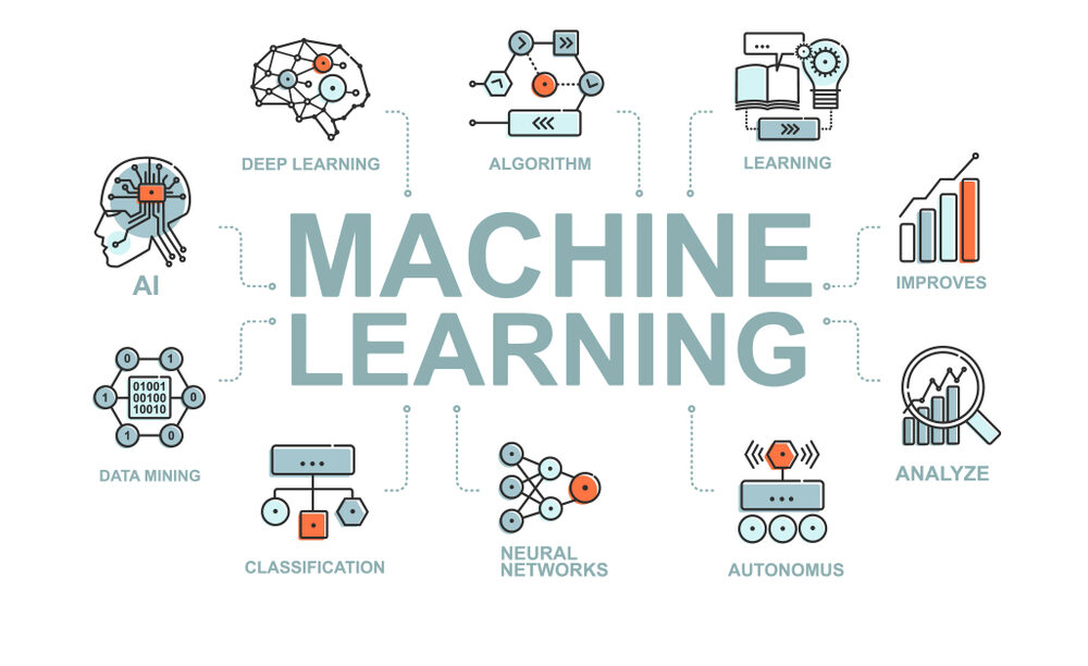
Key Components of Machine Learning:#
Algorithms and Statisatical Analysis#
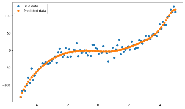
These are the foundational mathematical models or procedures that enable computers to learn from data. Algorithms are designed to identify patterns, correlations, and structures within the data to make predictions or decisions. This involves statisataical analysis on the data relationship to predict unseen values based on past observation.
By examining historical data patterns and relationships, these algorithms can predict or estimate future outcomes or unseen values based on past observations. This predictive capability enables ML models to make informed decisions or generate accurate forecasts.
Once the model has learned from the training data, it aims to generalize its learned patterns to new, unseen data. The goal is for the model to make accurate predictions or decisions when presented with examples it hasn’t encountered during training.
Training Data#

Machine Learning algorithms require large volumes of data to learn from. This data, also known as training data, comprises examples, features, or attributes that the algorithm uses to understand relationships and patterns.
Training data consists of a collection of examples or instances, each representing a specific data point. Each example in the training data is associated with a set of features or attributes. These features describe the characteristics or properties of the data. In an image, features might include pixel values, color histograms, or textures.
Machine Learning algorithms learn from the patterns and relationships present in the training data. By analyzing these examples and their associated features, the algorithms discern correlations, dependencies, and structures.
Learning and Adaptation#
.jpeg)
The learning process involves training algorithms on datasets containing examples or instances with associated features and labels. During this training phase, the algorithms iteratively adjust their internal parameters or structures by analyzing the data relationships. Through optimization techniques like gradient descent or other optimization algorithms, these models learn to minimize errors or discrepancies between predicted outcomes and actual observations.
Once trained, Machine Learning models generalize their acquired knowledge to new, unseen data. They apply the patterns and relationships learned during training to make predictions or decisions on previously unseen examples. This generalization ability is a critical aspect that determines the model’s performance in real-world scenarios.
Types of Machine Learning:#
Machine learning uses programmed algorithms that receive and analyse input data to predict output values within an acceptable range. As new data is fed to these algorithms, they learn and optimise their operations to improve performance, developing intelligence over time.
There are 3 main types of machine learning algorithms: supervised learning, unsupervised learning and reinforcement learning.

Supervised Learning#
In supervised learning, the machine is taught by example. The operator provides the machine learning algorithm with a known dataset that includes desired inputs and outputs, and the algorithm must find a method to determine how to arrive at those inputs and outputs. While the operator knows the correct answers to the problem, the algorithm identifies patterns in data, learns from observations and makes predictions. The algorithm makes predictions and is corrected by the operator – and this process continues until the algorithm achieves a high level of accuracy/performance.
Under the umbrella of supervised learning fall: Classification, Regression and Forecasting.
Classification: In classification tasks, the machine learning program must draw a conclusion from observed values and determine to what category new observations belong. For example, when filtering emails as ‘spam’ or ‘not spam’, the program must look at existing observational data and filter the emails accordingly.
Regression: In regression tasks, the machine learning program must estimate – and understand – the relationships among variables. Regression analysis focuses on one dependent variable and a series of other changing variables – making it particularly useful for prediction and forecasting.
Forecasting: Forecasting is the process of making predictions about the future based on the past and present data, and is commonly used to analyse trends.
Exploring Machine Learning in Cybersecurity#
As we embark on our exploration of machine learning, let’s begin with an illustrative example showcasing the potential impact of machine learning in cybersecurity.
Spam Classification#
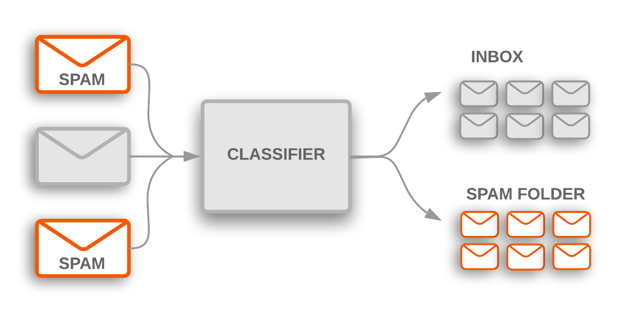
In this example, we used text classification to determined whether the messages is spam or not. We used NLP methods to prepare and clean our text data (tokenization, remove stop words, stemming) and different machine learning algorithms to get more accurate predictions. The following classification algorithms have been used: Logistic Regression, Naive Bayes, Support Vector Machine (SVM), Random Forest, Stochastic Gradient Descent and Gradient Boosting.
Dataset#
The dataset comes from SMS Spam Collection that can be find at https://www.kaggle.com/uciml/sms-spam-collection-dataset.
This SMS Spam Collection is a set of SMS tagged messages that have been collected for SMS Spam research. It comprises one set of SMS messages in English of 5,574 messages, which is tagged acording being ham (legitimate) or spam.
We begin by first importing several libraries for data analysis, natural language processing (NLP), and machine learning in Python. Some of the libraries imported include pandas for data manipulation, numpy for numerical operations, matplotlib and seaborn for data visualization, and nltk for natural language processing tasks like tokenization and stemming. Additionally, we import functions from scikit-learn (sklearn) for machine learning tasks such as model selection, creating pipelines, feature extraction, and various classification algorithms.
Moreover, we downloads the stopwords corpus from NLTK (Natural Language Toolkit), which contains a list of common words often considered irrelevant in text analysis tasks.
import pandas as pd
import numpy as np
import matplotlib.pyplot as plt
import seaborn as sns

import re
import nltk
from nltk.corpus import stopwords
from nltk.stem import PorterStemmer
from nltk.tokenize import sent_tokenize, word_tokenize

from sklearn.model_selection import train_test_split
from sklearn.pipeline import Pipeline
from sklearn.feature_extraction.text import CountVectorizer, TfidfTransformer

# from imblearn.over_sampling import SMOTE

from sklearn.linear_model import LogisticRegression
from sklearn.naive_bayes import MultinomialNB
from sklearn.ensemble import RandomForestClassifier
from sklearn.svm import LinearSVC
from sklearn.linear_model import SGDClassifier
from sklearn.ensemble import GradientBoostingClassifier

from sklearn.metrics import confusion_matrix, accuracy_score, classification_report

nltk.download("stopwords")
None
[nltk_data] Downloading package stopwords to
[nltk_data]     /home/soraxas/nltk_data...
[nltk_data]   Unzipping corpora/stopwords.zip.
Next, we read a CSV file containing spam-related data, preprocesses it by removing unnecessary columns, renaming columns, converting categorical labels to numerical values, and creates a copy of the preprocessed DataFrame for further analysis or manipulation.
spam = pd.read_csv(
    "https://raw.githubusercontent.com/WSU-AI-CyberSecurity/data/master/spam.csv",
    encoding="latin-1",
)
spam.drop(["Unnamed: 2", "Unnamed: 3", "Unnamed: 4"], axis=1, inplace=True)
spam.rename(columns={"v1": "Class", "v2": "Text"}, inplace=True)
spam["Class"] = spam["Class"].map({"ham": 0, "spam": 1})

spam_ori = spam.copy()
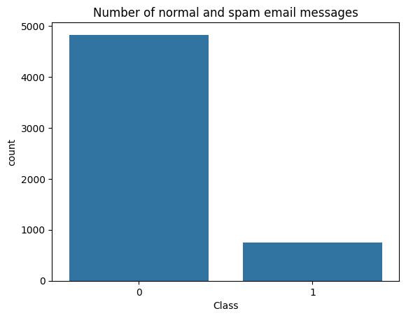
Let’s visualise the number of genuine and spam email#
sns.countplot(x="Class", data=spam)
plt.xlabel("Class")
plt.title("Number of normal and spam email messages")
Text(0.5, 1.0, 'Number of normal and spam email messages')
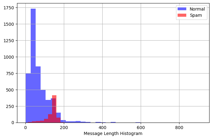
plt.figure(figsize=(8, 5))
spam[spam.Class == 0].Text.str.len().hist(
    bins=35, color="blue", label="Normal", alpha=0.6
)
spam[spam.Class == 1].Text.str.len().hist(color="red", label="Spam", alpha=0.6)
plt.legend()
plt.xlabel("Message Length Histogram")
Text(0.5, 0, 'Message Length Histogram')
def clean_text(words):
    """The function to clean text"""
    words = re.sub("[^a-zA-Z]", " ", words)
    text = words.lower().split()
    return " ".join(text)


def remove_stopwords(text):
    """The function to removing stopwords"""
    text = [word.lower() for word in text.split() if word.lower() not in stop_words]
    return " ".join(text)


def stemmer(stem_text):
    """The function to apply stemming"""
    stem_text = [porter.stem(word) for word in stem_text.split()]
    return " ".join(stem_text)


stop_words = stopwords.words("english")
porter = PorterStemmer()

spam["Text"] = spam["Text"].apply(clean_text)
spam.head()

spam["Text"] = spam["Text"].apply(remove_stopwords)
spam["Text"] = spam["Text"].apply(stemmer)
X = spam["Text"]
y = spam["Class"]
vect = CountVectorizer(min_df=5, ngram_range=(1, 2)).fit(X)
X_vec = vect.transform(X)

X_train, X_test, y_train, y_test = train_test_split(
    X_vec, y, test_size=0.2, random_state=0
)

model_lr = Pipeline(
    [
        ("tfidf", TfidfTransformer()),
        ("model", LogisticRegression()),
    ]
)

model_lr.fit(X_train, y_train)

ytest = np.array(y_test)
pred_y = model_lr.predict(X_test)
model_nb = Pipeline(
    [
        ("tfidf", TfidfTransformer()),
        ("model", MultinomialNB()),
    ]
)

model_nb.fit(X_train, y_train)

ytest = np.array(y_test)
pred = model_nb.predict(X_test)
def map_bool_to_checkmark(text):
    return "✔" if text else "✗"


count = 0

data = {"Email": [], "Is spam?": [], "predicted": []}
for idx, gt, pred in zip(y_test.index, y_test, pred_y):
    data["Email"].append(spam_ori.Text[idx])
    data["Is spam?"].append(map_bool_to_checkmark(gt))
    data["predicted"].append(map_bool_to_checkmark(pred))
    count += 1
    if count > 15:
        break

print("=========================\nFirst 15 results:\n=========================")
display(pd.DataFrame(data))
=========================
First 15 results:
=========================
| Is spam? | predicted | ||
|---|---|---|---|
| 0 | Aight should I just plan to come up later toni... | ✗ | ✗ |
| 1 | Was the farm open? | ✗ | ✗ |
| 2 | I sent my scores to sophas and i had to do sec... | ✗ | ✗ |
| 3 | Was gr8 to see that message. So when r u leavi... | ✗ | ✗ |
| 4 | In that case I guess I'll see you at campus lodge | ✗ | ✗ |
| 5 | Nothing will ever be easy. But don't be lookin... | ✗ | ✗ |
| 6 | If you were/are free i can give. Otherwise nal... | ✗ | ✗ |
| 7 | Hey i will be late... i'm at amk. Need to drin... | ✗ | ✗ |
| 8 | Hey are we going for the lo lesson or gym? | ✗ | ✗ |
| 9 | 85233 FREE>Ringtone!Reply REAL | ✔ | ✔ |
| 10 | \The world suffers a lot... Not because of the... | ✗ | ✗ |
| 11 | Hey!!! I almost forgot ... Happy B-day babe ! ... | ✗ | ✗ |
| 12 | I wish u were here. I feel so alone | ✗ | ✗ |
| 13 | sports fans - get the latest sports news str* ... | ✔ | ✔ |
| 14 | LMAO where's your fish memory when I need it? | ✗ | ✗ |
| 15 | Oh is it! Which brand? | ✗ | ✗ |
Terminologies#
Let us revisit some of the key terminology used in machine learning that we’ve glanced throught in our previous spam detection:
Features#
In machine learning, features refer to the individual measurable properties or characteristics used to represent the data. These features are the variables or attributes that are fed into a machine learning algorithm as inputs for making predictions or classifications. For instance, in a spam detection task for emails, features might include the frequency of certain words, email sender’s address, length of the email, etc. Each piece of data is represented by its features, and the quality and relevance of features greatly influence the performance of machine learning models.
Labels#
In supervised machine learning, labels are the outcomes or target variables that the model aims to predict. These are the answers or expected results that the model tries to learn from the input data. In a classification task like spam detection, labels could be binary categories such as spam or not spam assigned to each data point. In regression tasks, labels might be continuous numerical values that the model predicts. The model learns patterns in the features to predict the corresponding labels accurately.
Algorithms#
Machine learning algorithms are computational procedures or techniques used by models to learn patterns and relationships from data. These algorithms are the core components that enable machines to learn from experience or data and make predictions or decisions without explicit programming. Various types of algorithms exist across machine learning, such as regression algorithms (linear regression, polynomial regression), classification algorithms (decision trees, support vector machines, logistic regression), clustering algorithms (k-means, hierarchical clustering), and more. Each algorithm has its strengths, weaknesses, and suitable use cases based on the nature of the data and the problem being addressed.
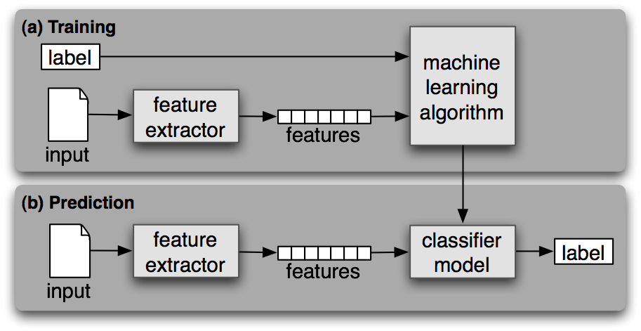
Understanding these terminologies is fundamental in grasping the concepts and workflows in machine learning. Features represent the input data, labels denote the output or target to be predicted, and algorithms are the methods/models that learn from the input-output pairs to make predictions or uncover patterns in the data. We use these in both our training and prediction procedure in our ML pipeline.
Evaulation Metrics#
One thing that we should always keep in our mind when building ML models is how to assess how good is my model?
Performance metrics in machine learning evaluate the effectiveness of a model’s predictions. They provide insights into how well a model performs in solving a particular problem. Here are some essential performance metrics:
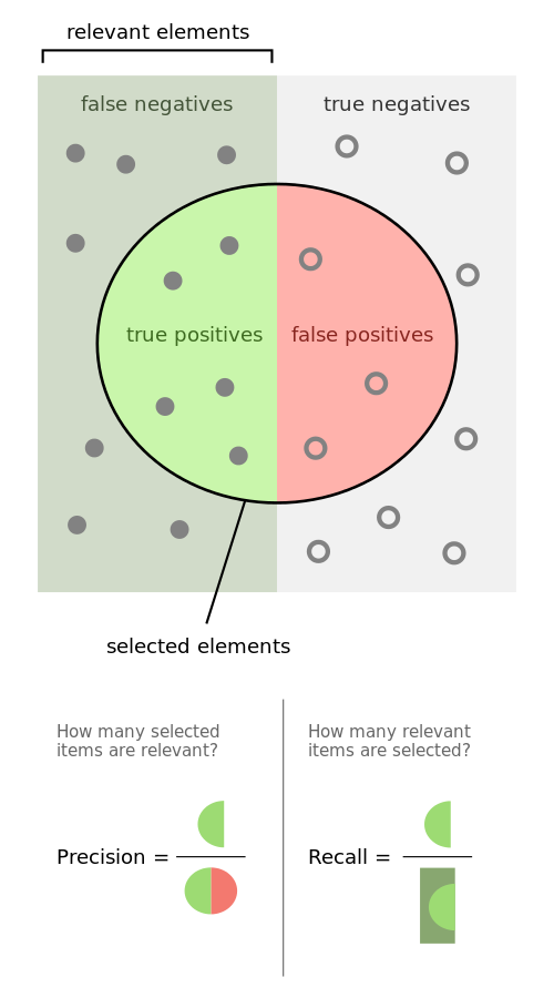
Accuracy: This metric measures the overall correctness of predictions made by a model. It calculates the ratio of correctly predicted instances to the total number of instances. It’s represented as:
\[\text{Accuracy} = \frac{\text{Number of Correct Predictions}}{\text{Total Number of Predictions}} \times 100\% \]While accuracy is a commonly used metric, it might not be suitable for imbalanced datasets where one class dominates the other. In such cases, other metrics become more informative.
Precision: Precision measures the accuracy of positive predictions made by the model. It quantifies the ratio of correctly predicted positive instances (true positives) to the total predicted positive instances (true positives + false positives). Precision is calculated as:
\[\text{Precision} = \frac{\text{True Positives}}{\text{True Positives + False Positives}}\]Precision is valuable when the cost of false positives is high. For instance, in a spam detection system, precision indicates the proportion of correctly classified spam emails among all emails flagged as spam.
Recall (Sensitivity): Recall measures the model’s ability to correctly identify all positive instances. It calculates the ratio of correctly predicted positive instances (true positives) to the total actual positive instances (true positives + false negatives). Mathematically, recall is given by:
\[\text{Recall} = \frac{\text{True Positives}}{\text{True Positives + False Negatives}}\]Recall is crucial when it’s important to capture all positive instances, even if some false positives occur. For example, in a medical diagnosis system, recall indicates the proportion of actual positive cases correctly identified among all positive cases.
F1 Score: The F1 score is the harmonic mean of precision and recall. It provides a balanced measure between precision and recall, considering both false positives and false negatives. F1 score is calculated as:
\[\text{F1 Score} = 2 \times \frac{\text{Precision} \times \text{Recall}}{\text{Precision + Recall}}\]F1 score is useful when you want to consider both precision and recall simultaneously. It’s a good metric for evaluating models on imbalanced datasets where one class significantly outnumbers the other.
These metrics help in understanding different aspects of a model’s performance. Accuracy provides an overall view, while precision, recall, and F1 score offer insights into specific aspects of model behavior, aiding in making informed decisions about the model’s suitability for a particular task. Choosing the appropriate metric depends on the specific goals and requirements of the problem being addressed.

We can now to the pre-built function from scikit-learn to compute these metric from our previous spam detection problem
from sklearn.metrics import accuracy_score, precision_score, recall_score, f1_score
from IPython.display import display, Math

# Calculate accuracy
accuracy = accuracy_score(y_test, pred_y)
display(Math(f"Accuracy: {accuracy*100:.2f}\%"))

# Calculate precision
precision = precision_score(y_test, pred_y)
display(Math(f"Precision: {precision*100:.2f}\%"))

# Calculate recall
recall = recall_score(y_test, pred_y)
display(Math(f"Recall: {recall*100:.2f}\%"))

# Calculate F1 score
f1 = f1_score(y_test, pred_y)
display(Math(f"F1-Score: {f1*100:.2f}\%"))

