Module 3: Data Preprocessing and Features Selection

Welcome to Module 3 of our learning journey! In this segment, we’ll delve into the critical aspects of Data Preprocessing and Feature Selection.

As aspiring data enthusiasts, you’ve likely realized that the journey from raw data to meaningful insights involves careful preparation and strategic selection. This module is designed to equip you with the essential skills to transform raw, messy data into a refined and feature-rich dataset, setting the stage for robust machine learning models.

Key Objectives:

Data cleaning and imputation are essential steps in the data preprocessing pipeline for several reasons:

1. Handling Missing Data:

   Real-world datasets often contain missing values due to various reasons such as measurement errors, system failures, or human error. Data cleaning and imputation techniques address these gaps, ensuring a complete and usable dataset.

2. Ensuring Data Quality:

   Inaccurate or inconsistent data can significantly impact the performance and reliability of machine learning models. Cleaning the data involves identifying and rectifying errors, ensuring the overall quality and integrity of the dataset.

3. Mitigating Outliers:

   Outliers, or extreme values, can distort statistical analyses and model predictions. Data cleaning involves identifying and handling outliers appropriately, preventing them from unduly influencing the model’s behavior.

4. Improving Model Performance:

   Machine learning algorithms often struggle with missing values and outliers. By cleaning and imputing data, the dataset becomes more suitable for model training, leading to improved performance and generalization on new, unseen data.

5. Enhancing Data Interpretability:

   Clean and well-imputed data fosters a better understanding of the underlying patterns and relationships. Researchers and analysts can trust the results and interpretations derived from a dataset that has undergone thorough cleaning and imputation.

6. Meeting Assumptions of Statistical Methods:

   Many statistical methods assume certain characteristics of the data, such as normal distribution or absence of missing values. Data cleaning ensures that the dataset adheres to these assumptions, allowing for the accurate application of statistical techniques.

7. Building Trust in Results:

   Stakeholders, decision-makers, and users of the machine learning model rely on accurate and trustworthy results. Data cleaning and imputation contribute to the credibility of the model’s outcomes, fostering trust in the decision-making process.

8. Reducing Bias and Error:

   Incomplete or biased datasets can lead to skewed and inaccurate model predictions. Data cleaning minimizes bias, ensuring that the model is trained on a representative and unbiased set of features.

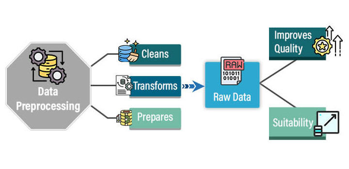
Why Data Preprocessing Matters:

Raw data seldom fits neatly into the algorithms we love to employ. Data preprocessing is the unsung hero that transforms raw data into a well-behaved companion, ensuring your models can extract meaningful patterns and insights.

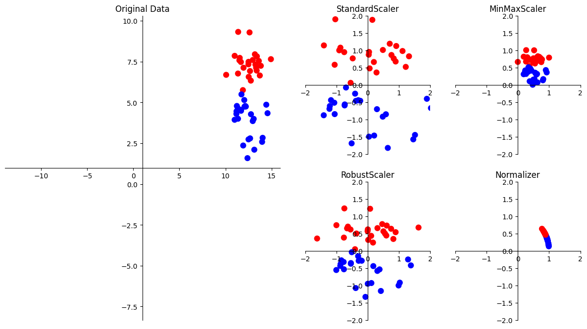
Visualising scaling methods

Let us visulaise what does scaling methods do to the input data. The following are some of the popular preprocessing methods in the sklearn library.

The four preprocessing methods—StandardScaler, MinMaxScaler, Normalizer, and RobustScaler—from scikit-learn’s preprocessing module serve different purposes in preparing and scaling data for machine learning models. Here’s an overview of each:

1. StandardScaler:

   • Method: StandardScaler standardizes features by removing the mean and scaling to unit variance.

   • Usage: It transforms features so that they have a mean of 0 and a standard deviation of 1.

   • When to Use: Suitable for algorithms that assume features follow a Gaussian distribution and for ensuring consistent scales for features.

2. MinMaxScaler:

   • Method: MinMaxScaler scales features to a specified range, typically between 0 and 1.

   • Usage: It transforms features, maintaining the original data’s shape while scaling it to a specified range.

   • When to Use: Useful when features need to be on a similar scale, but you want to preserve the original distribution.

3. Normalizer:

   • Method: Normalizer scales each sample (row) independently, such that the Euclidean norm (L2 norm) of each row is equal to 1.

   • Usage: It normalizes samples to a unit norm, useful when the direction of each data point is more important than its magnitude.

   • When to Use: Appropriate when working with datasets where the magnitude of the individual samples is crucial.

4. RobustScaler:

   • Method: RobustScaler scales features using statistics that are robust to outliers. It uses the median and the interquartile range (IQR).

   • Usage: It scales features while being less affected by outliers compared to StandardScaler.

   • When to Use: Suitable when the dataset contains outliers and a more robust scaling method is needed.

In summary, these preprocessing methods provide flexibility in handling different types of data and scaling requirements. The choice of scaler depends on the characteristics of the data and the assumptions of the machine learning algorithm being used.

In practice, StandardScaler is the most typical approach as it requires less assumptions and works well in most scenarios.

!pip install kaleido

Collecting kaleido
  Downloading kaleido-0.2.1-py2.py3-none-manylinux1_x86_64.whl (79.9 MB)
     ━━━━━━━━━━━━━━━━━━━━━━━━━━━━━━━━━━━━━━━━ 79.9/79.9 MB 7.5 MB/s eta 0:00:00m eta 0:00:01[36m0:00:01
?25hInstalling collected packages: kaleido
Successfully installed kaleido-0.2.1

import matplotlib.pyplot as plt
import numpy as np
from sklearn.datasets import make_blobs
from sklearn.preprocessing import StandardScaler, MinMaxScaler, Normalizer, RobustScaler

cm2 = "bwr"

X, y = make_blobs(n_samples=50, centers=2, random_state=4, cluster_std=1)
X += 3

plt.figure(figsize=(15, 8))
main_ax = plt.subplot2grid((2, 4), (0, 0), rowspan=2, colspan=2)

main_ax.scatter(X[:, 0], X[:, 1], c=y, cmap=cm2, s=60)
maxx = np.abs(X[:, 0]).max()
maxy = np.abs(X[:, 1]).max()

main_ax.set_xlim(-maxx + 1, maxx + 1)
main_ax.set_ylim(-maxy + 1, maxy + 1)
main_ax.set_title("Original Data")
other_axes = [plt.subplot2grid((2, 4), (i, j)) for j in range(2, 4) for i in range(2)]

for ax, scaler in zip(
    other_axes,
    [StandardScaler(), RobustScaler(), MinMaxScaler(), Normalizer(norm="l2")],
):
    X_ = scaler.fit_transform(X)
    ax.scatter(X_[:, 0], X_[:, 1], c=y, cmap=cm2, s=60)
    ax.set_xlim(-2, 2)
    ax.set_ylim(-2, 2)
    ax.set_title(type(scaler).__name__)

other_axes.append(main_ax)

for ax in other_axes:
    ax.spines["left"].set_position("center")
    ax.spines["right"].set_color("none")
    ax.spines["bottom"].set_position("center")
    ax.spines["top"].set_color("none")
    ax.xaxis.set_ticks_position("bottom")
    ax.yaxis.set_ticks_position("left")

Navigating the Module:

We encourage you to actively participate in exercises, experiment with the provided code snippets, and explore real-world scenarios. Don’t hesitate to ask questions and engage with your peers – learning is a collaborative journey!

So, gear up for an illuminating exploration of Data Preprocessing and Feature Selection. Let’s refine our data and set the stage for machine learning success!

Imports

Let’s begin by importing some of the common modules that we’ll be using today.

import sys
import time

import matplotlib.pyplot as plt

%matplotlib inline
import numpy as np
import pandas as pd
from IPython.display import HTML

from IPython.display import display

# Classifiers and regressors
from sklearn.dummy import DummyClassifier, DummyRegressor

# Preprocessing and pipeline
from sklearn.impute import SimpleImputer

# train test split and cross validation
from sklearn.model_selection import cross_val_score, cross_validate, train_test_split
from sklearn.neighbors import KNeighborsClassifier, KNeighborsRegressor
from sklearn.pipeline import Pipeline
from sklearn.preprocessing import (
    MinMaxScaler,
    OneHotEncoder,
    OrdinalEncoder,
    StandardScaler,
)
from sklearn.svm import SVC
from sklearn.tree import DecisionTreeClassifier
from sklearn.metrics.pairwise import euclidean_distances
import plotly.express as pe

pd.set_option("display.max_colwidth", 200)

Example: \(k\)-nearest neighbours on the Spotify dataset

• Yesterday in our workshop, we’ve used DecisionTreeClassifier, and today we will use the same model to predict whether the user would like a particular song or not.

• Intuition: To predict whether the user likes a particular song or not (query point)

  • find the songs that are closest to the query point

  • let them vote on the target

  • take the majority vote as the target for the query point

We are going to use the Spotify Song Attributes dataset from Kaggle.

spotify_df = pd.read_csv(
    "https://raw.githubusercontent.com/WSU-AI-CyberSecurity/data/master/spotify.csv",
    index_col=0,
)
train_df, test_df = train_test_split(spotify_df, test_size=0.20, random_state=123)
X_train, y_train = (
    train_df.drop(columns=["song_title", "artist", "target"]),
    train_df["target"],
)
X_test, y_test = (
    test_df.drop(columns=["song_title", "artist", "target"]),
    test_df["target"],
)

Let us first define a baseline dummy classifier:

The DummyClassifier in scikit-learn is a simple, baseline classifier used for reference and comparison in machine learning tasks. It allows you to create a dummy or baseline model that serves as a basic benchmark to evaluate the performance of more sophisticated models. The primary purpose of DummyClassifier is to provide a minimalistic model to compare against when assessing the effectiveness of your machine learning models.

• In our code, we use most_frequent, which means that it will always just predict the most frequent class.

dummy = DummyClassifier(strategy="most_frequent")
scores = cross_validate(dummy, X_train, y_train, return_train_score=True)
print("Mean validation score %0.3f" % (np.mean(scores["test_score"])))
pd.DataFrame(scores)

Mean validation score 0.508

	fit_time	score_time	test_score	train_score
0	0.000490	0.000365	0.507740	0.507752
1	0.000410	0.000307	0.507740	0.507752
2	0.000403	0.000473	0.507740	0.507752
3	0.000404	0.000447	0.506211	0.508133
4	0.000564	0.000638	0.509317	0.507359

knn = KNeighborsClassifier()
scores = cross_validate(knn, X_train, y_train, return_train_score=True)
print("Mean validation score %0.3f" % (np.mean(scores["test_score"])))
pd.DataFrame(scores)

Mean validation score 0.546

	fit_time	score_time	test_score	train_score
0	0.002164	0.010995	0.563467	0.717829
1	0.002701	0.007564	0.535604	0.721705
2	0.002035	0.005789	0.529412	0.708527
3	0.001661	0.005154	0.537267	0.721921
4	0.001440	0.005330	0.562112	0.711077

two_songs = X_train.sample(2, random_state=42)
print(
    "===== This is the distance of the two song by considering the following features ====="
)
display(two_songs)
print("===== Distance: =====")
euclidean_distances(two_songs)

===== This is the distance of the two song by considering the following features =====

	acousticness	danceability	duration_ms	energy	instrumentalness	key	liveness	loudness	mode	speechiness	tempo	time_signature	valence
842	0.229000	0.494	147893	0.666	0.000057	9	0.0469	-9.743	0	0.0351	140.832	4.0	0.704
654	0.000289	0.771	227143	0.949	0.602000	8	0.5950	-4.712	1	0.1750	111.959	4.0	0.372

===== Distance: =====

array([[    0.        , 79250.00543825],
       [79250.00543825,     0.        ]])

Let’s consider only two features: duration_ms and tempo.

two_songs_subset = two_songs[["duration_ms", "tempo"]]
print(
    "===== This is the distance of the two song by considering the following features ====="
)
display(two_songs_subset)
print("===== Distance: =====")
euclidean_distances(two_songs_subset)

===== This is the distance of the two song by considering the following features =====

	duration_ms	tempo
842	147893	140.832
654	227143	111.959

===== Distance: =====

array([[    0.        , 79250.00525962],
       [79250.00525962,     0.        ]])

Do you see any problem?

The distance of the two song, regardless of whether we are considering all features (13 total), or only a subset of features (only 2), have essentially the same value (79250.0054….)

• The distance is completely dominated by the the features with larger values

• The features with smaller values are being ignored.

• Does it matter?

  • Yes! Scale is based on how data was collected.

  • Features on a smaller scale can be highly informative and there is no good reason to ignore them.

  • We want our model to be robust and not sensitive to the scale.

• Was this a problem for decision trees?

Scaling using scikit-learn’s StandardScaler

• We’ll use scikit-learn’s StandardScaler, which is a transformer.

• Only focus on the syntax for now. We’ll talk about scaling in a bit.

from sklearn.preprocessing import StandardScaler

scaler = StandardScaler()  # create feature trasformer object
scaler.fit(X_train)  # fitting the transformer on the train split
X_train_scaled = scaler.transform(X_train)  # transforming the train split
X_test_scaled = scaler.transform(X_test)  # transforming the test split

X_train  # original X_train

	acousticness	danceability	duration_ms	energy	instrumentalness	key	liveness	loudness	mode	speechiness	tempo	time_signature	valence
1505	0.004770	0.585	214740	0.614	0.000155	10	0.0762	-5.594	0	0.0370	114.059	4.0	0.2730
813	0.114000	0.665	216728	0.513	0.303000	0	0.1220	-7.314	1	0.3310	100.344	3.0	0.0373
615	0.030200	0.798	216585	0.481	0.000000	7	0.1280	-10.488	1	0.3140	127.136	4.0	0.6400
319	0.106000	0.912	194040	0.317	0.000208	6	0.0723	-12.719	0	0.0378	99.346	4.0	0.9490
320	0.021100	0.697	236456	0.905	0.893000	6	0.1190	-7.787	0	0.0339	119.977	4.0	0.3110
...	...	...	...	...	...	...	...	...	...	...	...	...	...
2012	0.001060	0.584	274404	0.932	0.002690	1	0.1290	-3.501	1	0.3330	74.976	4.0	0.2110
1346	0.000021	0.535	203500	0.974	0.000149	10	0.2630	-3.566	0	0.1720	116.956	4.0	0.4310
1406	0.503000	0.410	256333	0.648	0.000000	7	0.2190	-4.469	1	0.0362	60.391	4.0	0.3420
1389	0.705000	0.894	222307	0.161	0.003300	4	0.3120	-14.311	1	0.0880	104.968	4.0	0.8180
1534	0.623000	0.470	394920	0.156	0.187000	2	0.1040	-17.036	1	0.0399	118.176	4.0	0.0591

1613 rows × 13 columns

Let’s examine transformed value of the energy feature in the first row.

X_train["energy"].iloc[0]

0.614

(X_train["energy"].iloc[0] - np.mean(X_train["energy"])) / X_train["energy"].std()

-0.3180174485124284

pd.DataFrame(X_train_scaled, columns=X_train.columns, index=X_train.index).head().round(
    3
)

	acousticness	danceability	duration_ms	energy	instrumentalness	key	liveness	loudness	mode	speechiness	tempo	time_signature	valence
1505	-0.698	-0.195	-0.399	-0.318	-0.492	1.276	-0.738	0.396	-1.281	-0.618	-0.294	0.139	-0.908
813	-0.276	0.296	-0.374	-0.796	0.598	-1.487	-0.439	-0.052	0.781	2.728	-0.803	-3.781	-1.861
615	-0.600	1.111	-0.376	-0.947	-0.493	0.447	-0.400	-0.879	0.781	2.535	0.191	0.139	0.576
319	-0.307	1.809	-0.654	-1.722	-0.492	0.170	-0.763	-1.461	-1.281	-0.609	-0.840	0.139	1.825
320	-0.635	0.492	-0.131	1.057	2.723	0.170	-0.458	-0.176	-1.281	-0.653	-0.074	0.139	-0.754

fit and transform paradigm for transformers

• sklearn uses fit and transform paradigms for feature transformations.

• We fit the transformer on the train split and then transform the train split as well as the test split.

• We apply the same transformations on the test split.

sklearn API summary: estimators

Suppose model is a classification or regression model.

model.fit(X_train, y_train)
X_train_predictions = model.predict(X_train)
X_test_predictions = model.predict(X_test)

The StandardScaler from scikit-learn is used to transform and standardize features by removing the mean and scaling to unit variance. Applying StandardScaler is beneficial for several reasons:

• Sandardization ensures that all features have a mean of 0 and a standard deviation of 1. This normalization is especially important for algorithms that rely on distance metrics, such as k-Nearest Neighbors or Support Vector Machines. It prevents features with larger scales from dominating the learning process.

• Standardizing features helps in comparing the relative importance of different features. It ensures that the coefficients or weights associated with each feature reflect their impact in a more meaningful way. Robustness to Outliers:

• Standardization is less influenced by outliers compared to some other scaling methods. It is based on the mean and standard deviation, which are less sensitive to extreme values.

• Do you expect DummyClassifier results to change after scaling the data?

• Let’s check whether scaling makes any difference for \(k\)-NNs.

knn_unscaled = KNeighborsClassifier()
knn_unscaled.fit(X_train, y_train)
print("Train score: %0.3f" % (knn_unscaled.score(X_train, y_train)))
print("Test score: %0.3f" % (knn_unscaled.score(X_test, y_test)))

Train score: 0.726
Test score: 0.552

knn_scaled = KNeighborsClassifier()
knn_scaled.fit(X_train_scaled, y_train)
print("Train score: %0.3f" % (knn_scaled.score(X_train_scaled, y_train)))
print("Test score: %0.3f" % (knn_scaled.score(X_test_scaled, y_test)))

Train score: 0.798
Test score: 0.686

The scores with scaled data are better compared to the unscaled data in case of \(k\)-NNs.

Common preprocessing techniques

Some commonly performed feature transformation include:

• Imputation: Tackling missing values

• Scaling: Scaling of numeric features

• One-hot encoding: Tackling categorical variables

In the next part of this module, we’ll build an ML pipeline using Cellular Network Analysis Dataset. In the process, we will talk about different feature transformations and how can we apply them so that we do not violate the golden rule.

Dataset, splitting, and baseline

We’ll be working on Cellular Network Analysis Dataset to demonstrate these feature transformation techniques. The task is to predict network latency, given a number of features from the collected metrics

train_df, test_df = train_test_split(
    pd.read_csv(
        "https://raw.githubusercontent.com/WSU-AI-CyberSecurity/data/master/signal_metrics.csv"
    ),
    test_size=0.1,
    random_state=123,
)

display(train_df.head())

	Timestamp	Locality	Latitude	Longitude	Signal Strength (dBm)	Signal Quality (%)	Data Throughput (Mbps)	Latency (ms)	Network Type	BB60C Measurement (dBm)	srsRAN Measurement (dBm)	BladeRFxA9 Measurement (dBm)
11286	2023-05-29 23:44:54.012478	Patliputra Colony	25.573834	85.174773	-88.823204	0.0	2.633925	118.470369	LTE	-90.679320	-97.310913	-91.341579
11445	2023-05-30 08:01:00.429985	Anandpuri	25.459679	85.100593	-84.338977	0.0	8.230689	62.104584	4G	-85.669232	-90.443197	-83.662386
8991	2023-05-25 00:24:06.665443	Kidwaipuri	25.718163	85.164846	-95.165973	0.0	27.416884	39.535036	5G	-92.364076	-101.027782	-92.289394
13062	2023-06-02 20:06:19.279726	Rajendra Nagar	25.646589	85.123178	-82.277196	0.0	2.681432	128.228075	LTE	-78.858775	-89.006250	-84.283168
4151	2023-05-14 12:42:29.428123	Kidwaipuri	25.687754	85.008608	-89.665566	0.0	4.607886	66.139469	4G	-90.044765	-96.717788	-87.254787

Let’s have a look at our dataset attributes and the kind of features that it contains:

train_df.info()

<class 'pandas.core.frame.DataFrame'>
Index: 15146 entries, 11286 to 15725
Data columns (total 12 columns):
 #   Column                        Non-Null Count  Dtype  
---  ------                        --------------  -----  
 0   Timestamp                     15146 non-null  object 
 1   Locality                      15146 non-null  object 
 2   Latitude                      15146 non-null  float64
 3   Longitude                     15146 non-null  float64
 4   Signal Strength (dBm)         15146 non-null  float64
 5   Signal Quality (%)            15146 non-null  float64
 6   Data Throughput (Mbps)        15146 non-null  float64
 7   Latency (ms)                  15146 non-null  float64
 8   Network Type                  15146 non-null  object 
 9   BB60C Measurement (dBm)       15146 non-null  float64
 10  srsRAN Measurement (dBm)      15146 non-null  float64
 11  BladeRFxA9 Measurement (dBm)  15146 non-null  float64
dtypes: float64(9), object(3)
memory usage: 1.5+ MB

train_df = train_df.drop(columns=["Timestamp", "Locality"])
test_df = test_df.drop(columns=["Timestamp", "Locality"])

EDA

train_df.info()

<class 'pandas.core.frame.DataFrame'>
Index: 15146 entries, 11286 to 15725
Data columns (total 10 columns):
 #   Column                        Non-Null Count  Dtype  
---  ------                        --------------  -----  
 0   Latitude                      15146 non-null  float64
 1   Longitude                     15146 non-null  float64
 2   Signal Strength (dBm)         15146 non-null  float64
 3   Signal Quality (%)            15146 non-null  float64
 4   Data Throughput (Mbps)        15146 non-null  float64
 5   Latency (ms)                  15146 non-null  float64
 6   Network Type                  15146 non-null  object 
 7   BB60C Measurement (dBm)       15146 non-null  float64
 8   srsRAN Measurement (dBm)      15146 non-null  float64
 9   BladeRFxA9 Measurement (dBm)  15146 non-null  float64
dtypes: float64(9), object(1)
memory usage: 1.3+ MB

We have one categorical feature and all other features are numeric features.

train_df.describe()

	Latitude	Longitude	Signal Strength (dBm)	Signal Quality (%)	Data Throughput (Mbps)	Latency (ms)	BB60C Measurement (dBm)	srsRAN Measurement (dBm)	BladeRFxA9 Measurement (dBm)
count	15146.000000	15146.000000	15146.000000	15146.0	15146.000000	15146.000000	15146.000000	15146.000000	15146.000000
mean	25.594919	85.137158	-90.060175	0.0	16.116261	101.407733	-68.567118	-74.165153	-68.567884
std	0.089658	0.090057	5.399430	0.0	25.620021	55.980000	40.197141	43.377956	40.147603
min	25.414575	84.957936	-113.082820	0.0	1.000423	10.019527	-115.667514	-121.598760	-114.683401
25%	25.523497	85.064075	-93.595083	0.0	2.001390	50.430155	-94.022080	-101.224898	-93.744037
50%	25.595584	85.138149	-89.641736	0.0	2.992287	100.451793	-89.112998	-96.801157	-89.263101
75%	25.667371	85.209626	-86.117291	0.0	9.933834	150.029733	0.000000	0.000000	0.000000
max	25.773648	85.316994	-74.644848	0.0	99.985831	199.991081	0.000000	0.000000	0.000000

## (optional)
train_df.hist(bins=50, figsize=(20, 15))

array([[<Axes: title={'center': 'Latitude'}>,
        <Axes: title={'center': 'Longitude'}>,
        <Axes: title={'center': 'Signal Strength (dBm)'}>],
       [<Axes: title={'center': 'Signal Quality (%)'}>,
        <Axes: title={'center': 'Data Throughput (Mbps)'}>,
        <Axes: title={'center': 'Latency (ms)'}>],
       [<Axes: title={'center': 'BB60C Measurement (dBm)'}>,
        <Axes: title={'center': 'srsRAN Measurement (dBm)'}>,
        <Axes: title={'center': 'BladeRFxA9 Measurement (dBm)'}>]],
      dtype=object)

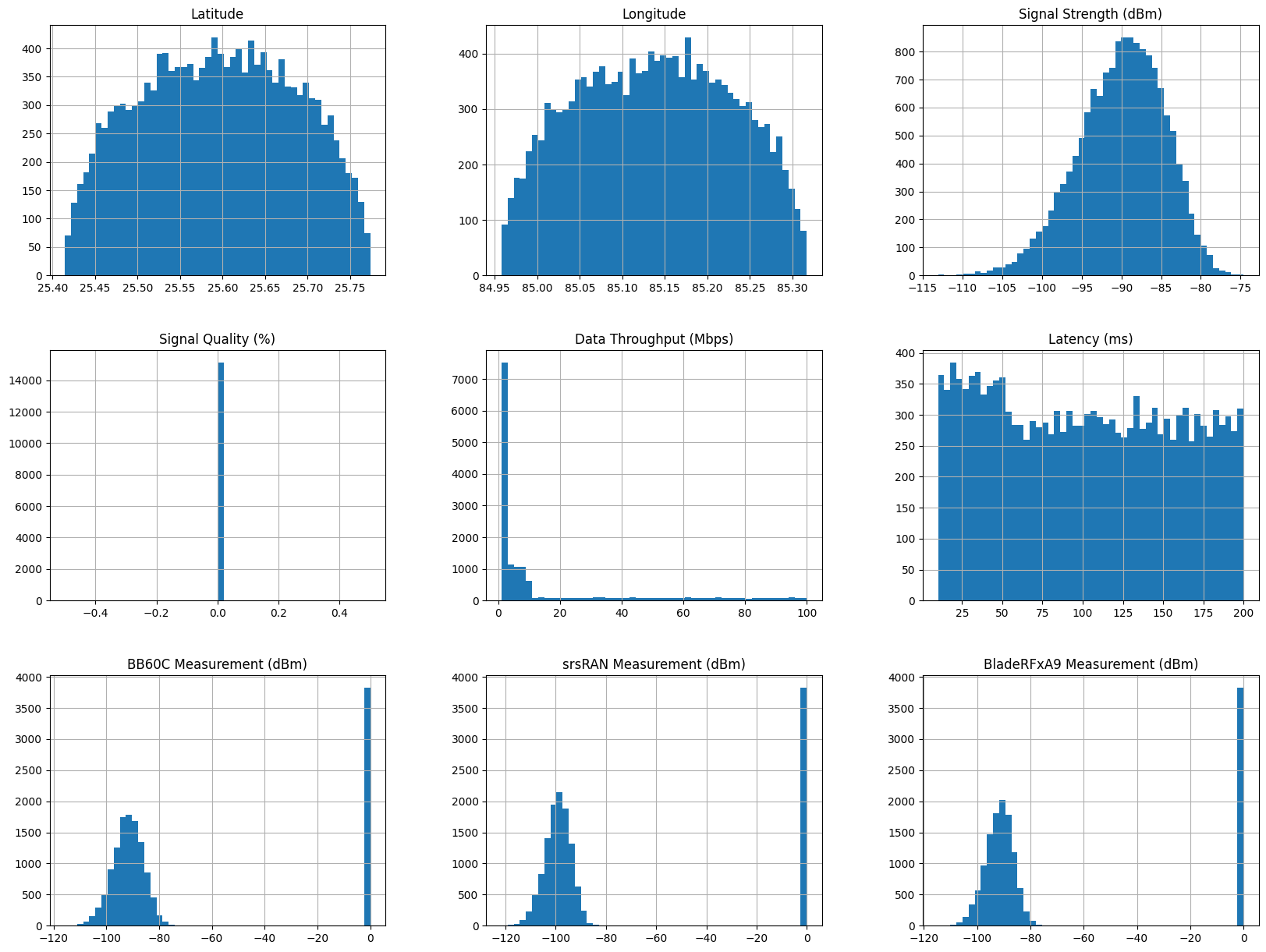
fig = pe.scatter_mapbox(
    train_df[train_df["Network Type"] == "5G"],
    lat="Latitude",
    lon="Longitude",
    mapbox_style="open-street-map",
    opacity=0.2,
    color="Signal Strength (dBm)",
    # color='BladeRFxA9 Measurement (dBm)',
)

fig.update_layout()
fig.update_layout(margin={"r": 0, "t": 0, "l": 0, "b": 0})

fig.show("png")

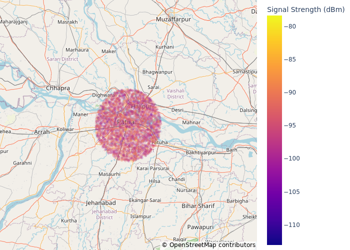
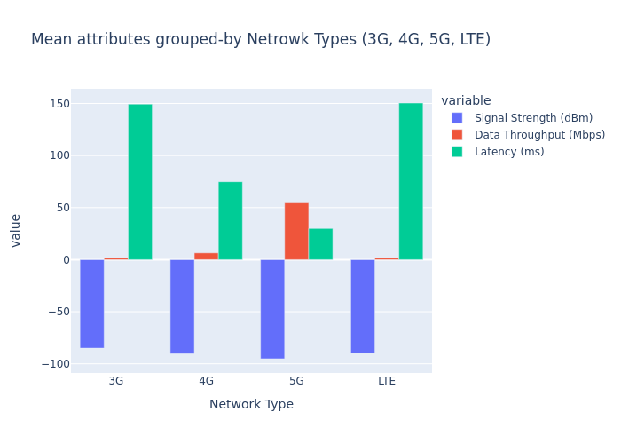
This visualisation indicates that all of the collected metrics are within certain radius of some area

fig = pe.bar(
    data_frame=train_df.groupby(["Network Type"]).mean().reset_index(),
    x="Network Type",
    y=["Signal Strength (dBm)", "Data Throughput (Mbps)", "Latency (ms)"],
    barmode="group",
    title="Mean attributes grouped-by Netrowk Types (3G, 4G, 5G, LTE)",
).show("png")

/home/soraxas/micromamba/envs/wsu/lib/python3.9/site-packages/plotly/express/_core.py:2065: FutureWarning:

When grouping with a length-1 list-like, you will need to pass a length-1 tuple to get_group in a future version of pandas. Pass `(name,)` instead of `name` to silence this warning.

What all transformations we need to apply on the dataset?

Here is what we see from the EDA.

• Scales are quite different across columns.

• Categorical variable Network Type

Read about preprocessing techniques implemented in scikit-learn.

X_train = train_df.drop(columns=["Latency (ms)", "Network Type"])
y_train = train_df["Latency (ms)"]

X_test = test_df.drop(columns=["Latency (ms)", "Network Type"])
y_test = test_df["Latency (ms)"]

Let’s first run our baseline model DummyRegressor

results_dict = {}  # dictionary to store our results for different models

def mean_std_cross_val_scores(model, X_train, y_train, **kwargs):
    """
    Returns mean and std of cross validation

    Parameters
    ----------
    model :
        scikit-learn model
    X_train : numpy array or pandas DataFrame
        X in the training data
    y_train :
        y in the training data

    Returns
    ----------
        pandas Series with mean scores from cross_validation
    """

    scores = cross_validate(model, X_train, y_train, **kwargs)

    mean_scores = pd.DataFrame(scores).mean()
    std_scores = pd.DataFrame(scores).std()
    out_col = []

    for i in range(len(mean_scores)):
        out_col.append((f"%0.3f (+/- %0.3f)" % (mean_scores[i], std_scores[i])))

    return pd.Series(data=out_col, index=mean_scores.index)

y_train

11286    118.470369
11445     62.104584
8991      39.535036
13062    128.228075
4151      66.139469
            ...    
96        31.932823
13435    109.640342
7763     101.868511
15377     21.659666
15725    177.697604
Name: Latency (ms), Length: 15146, dtype: float64

dummy = DummyRegressor(strategy="median")
results_dict["dummy"] = mean_std_cross_val_scores(
    dummy, X_train, y_train, return_train_score=True
)

/tmp/ipykernel_34641/4158382658.py:26: FutureWarning:

Series.__getitem__ treating keys as positions is deprecated. In a future version, integer keys will always be treated as labels (consistent with DataFrame behavior). To access a value by position, use `ser.iloc[pos]`

pd.DataFrame(results_dict)

	dummy
fit_time	0.001 (+/- 0.001)
score_time	0.000 (+/- 0.000)
test_score	-0.001 (+/- 0.000)
train_score	-0.000 (+/- 0.000)

Scaling

• This problem affects a large number of ML methods.

• A number of approaches to this problem. We are going to look into the most popular ones.

Approach	What it does	How to update \(X\) (but see below!)	sklearn implementation
standardization	sets sample mean to \(0\), s.d. to \(1\)	X -= np.mean(X,axis=0) X /=  np.std(X,axis=0)	StandardScaler()

scaler = StandardScaler()
X_train_scaled = scaler.fit_transform(X_train)
X_test_scaled = scaler.transform(X_test)
pd.DataFrame(X_train_scaled, columns=X_train.columns)

	Latitude	Longitude	Signal Strength (dBm)	Signal Quality (%)	Data Throughput (Mbps)	BB60C Measurement (dBm)	srsRAN Measurement (dBm)	BladeRFxA9 Measurement (dBm)
0	-0.235178	0.417697	0.229100	0.0	-0.526260	-0.550112	-0.533601	-0.567268
1	-1.508445	-0.406029	1.059628	0.0	-0.307800	-0.425470	-0.375273	-0.375988
2	1.374633	0.307469	-0.945649	0.0	0.441100	-0.592026	-0.619290	-0.590877
3	0.576312	-0.155235	1.441492	0.0	-0.524405	-0.256038	-0.342146	-0.391451
4	1.035463	-1.427470	0.073086	0.0	-0.449209	-0.534325	-0.519927	-0.465470
...	...	...	...	...	...	...	...	...
15141	-1.249304	0.776592	-1.054591	0.0	2.334350	-0.768915	-0.626568	-0.693106
15142	0.476210	-0.607609	-0.557700	0.0	-0.557237	-0.696676	-0.616269	-0.633682
15143	-0.753742	-1.671379	0.533930	0.0	-0.585827	-0.485844	-0.451067	-0.472370
15144	1.234431	-0.034641	-2.463528	0.0	0.052647	-0.826386	-0.863319	-0.896739
15145	1.171396	0.741267	0.508109	0.0	-0.578728	1.705827	1.709799	1.707951

15146 rows × 8 columns

knn = KNeighborsRegressor()
knn.fit(X_train_scaled, y_train)
knn.score(X_train_scaled, y_train)

0.7797007360451268

• Big difference in the KNN training performance after scaling the data.

• But we saw last week that training score doesn’t tell us much. We should look at the cross-validation score.

Feature transformations and the golden rule

Let’s try cross-validation with transformed data.

knn = KNeighborsRegressor()

scaler = StandardScaler()
scaler.fit(X_train)
X_train_scaled = scaler.transform(X_train)
X_test_scaled = scaler.transform(X_test)
scores = cross_validate(knn, X_train_scaled, y_train, return_train_score=True)
pd.DataFrame(scores)

	fit_time	score_time	test_score	train_score
0	0.007546	0.027821	0.669859	0.773023
1	0.005107	0.017332	0.657948	0.774226
2	0.005582	0.019061	0.657192	0.772506
3	0.005142	0.017042	0.646960	0.775659
4	0.005085	0.017823	0.647245	0.774178

• Do you see any problem here?

• Are we applying fit_transform on train portion and transform on validation portion in each fold?

  • Here you might be allowing information from the validation set to leak into the training step.

• You need to apply the SAME preprocessing steps to train/validation.

• With many different transformations and cross validation the code gets unwieldy very quickly.

• Likely to make mistakes and “leak” information.

• In these examples our test accuracies look fine, but our methodology is flawed.

• Implications can be significant in practice!

Pipelines

Can we do this in a more elegant and organized way?

• YES!! Using scikit-learn Pipeline.

• scikit-learn Pipeline allows you to define a “pipeline” of transformers with a final estimator.

Let’s combine the preprocessing and model with pipeline

### Simple example of a pipeline
from sklearn.pipeline import Pipeline

pipe = Pipeline(
    steps=[
        ("imputer", SimpleImputer(strategy="median")),
        ("scaler", StandardScaler()),
        ("regressor", KNeighborsRegressor()),
    ]
)

• Syntax: pass in a list of steps.

• The last step should be a model/classifier/regressor.

• All the earlier steps should be transformers.

Alternative and more compact syntax: make_pipeline

• Shorthand for Pipeline constructor

• Does not permit naming steps

• Instead the names of steps are set to lowercase of their types automatically; StandardScaler() would be named as standardscaler

from sklearn.pipeline import make_pipeline

pipe = make_pipeline(
    SimpleImputer(strategy="median"), StandardScaler(), KNeighborsRegressor()
)

pipe.fit(X_train, y_train)

Pipeline(steps=[('simpleimputer', SimpleImputer(strategy='median')),
                ('standardscaler', StandardScaler()),
                ('kneighborsregressor', KNeighborsRegressor())])

In a Jupyter environment, please rerun this cell to show the HTML representation or trust the notebook.
On GitHub, the HTML representation is unable to render, please try loading this page with nbviewer.org.

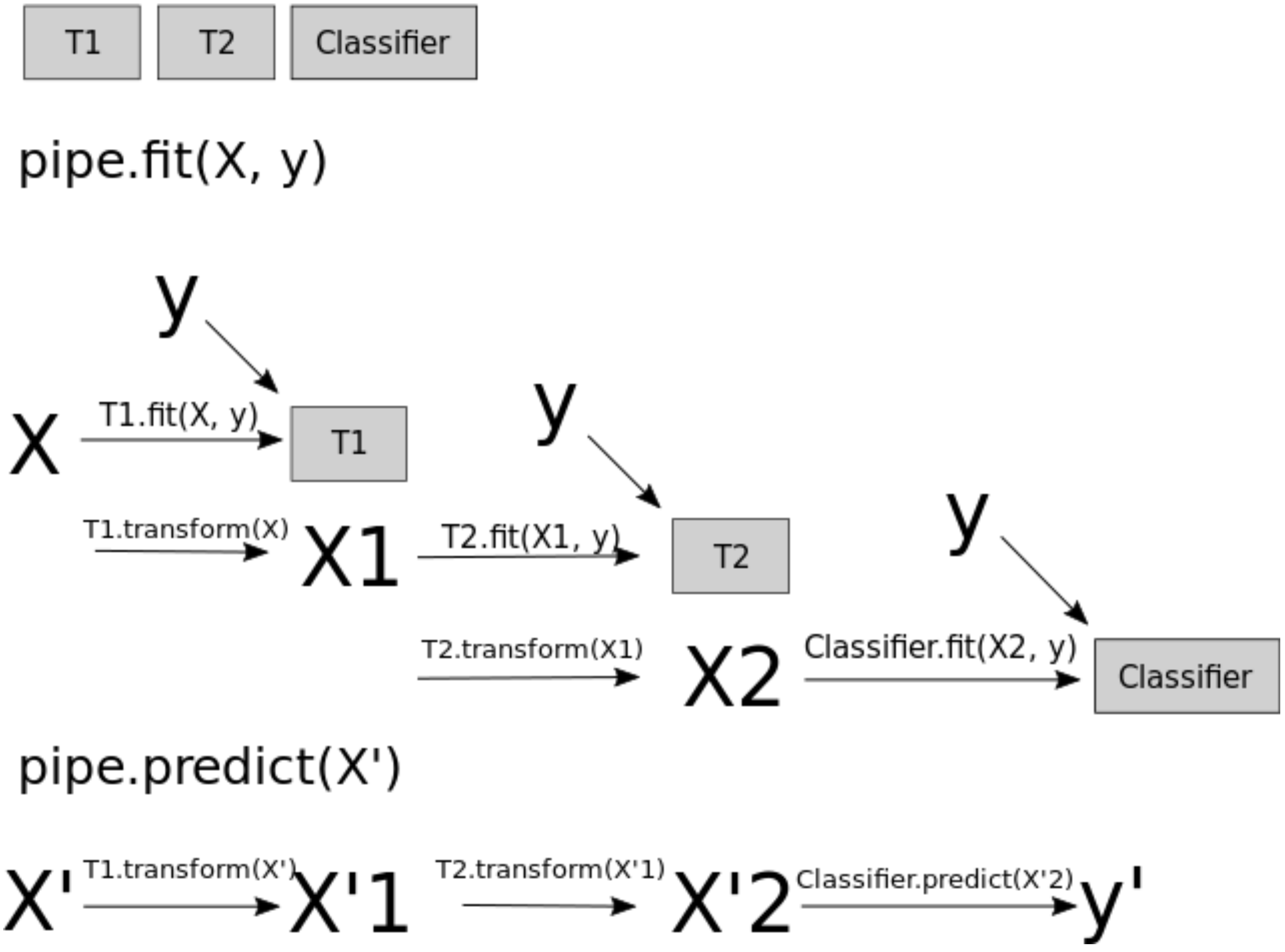
When you call fit on the pipeline, it carries out the following steps:

• Fit SimpleImputer on X_train

• Transform X_train using the fit SimpleImputer to create X_train

• Fit StandardScaler on X_train

• Transform X_train using the fit StandardScaler

• Fit the model (KNeighborsRegressor in our case)

pipe.predict(X_train)

array([120.28679471,  75.96071876,  29.21442221, ..., 142.46425035,
        44.20921845, 166.92819945])

Let’s try cross-validation with our pipeline

results_dict["imp + scaling + knn"] = mean_std_cross_val_scores(
    pipe, X_train, y_train, return_train_score=True
)
pd.DataFrame(results_dict).T

/tmp/ipykernel_34641/4158382658.py:26: FutureWarning:

Series.__getitem__ treating keys as positions is deprecated. In a future version, integer keys will always be treated as labels (consistent with DataFrame behavior). To access a value by position, use `ser.iloc[pos]`

	fit_time	score_time	test_score	train_score
dummy	0.001 (+/- 0.001)	0.000 (+/- 0.000)	-0.001 (+/- 0.000)	-0.000 (+/- 0.000)
imp + scaling + knn	0.013 (+/- 0.002)	0.018 (+/- 0.001)	0.656 (+/- 0.010)	0.774 (+/- 0.001)

Using a Pipeline takes care of applying the fit_transform on the train portion and only transform on the validation portion in each fold.

Categorical features

• Recall that we had dropped the categorical feature Network Type feature from the dataframe. But it could potentially be a useful feature in this task.

• Let’s create our X_train and and X_test again by keeping the feature in the data.

X_train

	Latitude	Longitude	Signal Strength (dBm)	Signal Quality (%)	Data Throughput (Mbps)	BB60C Measurement (dBm)	srsRAN Measurement (dBm)	BladeRFxA9 Measurement (dBm)
11286	25.573834	85.174773	-88.823204	0.0	2.633925	-90.679320	-97.310913	-91.341579
11445	25.459679	85.100593	-84.338977	0.0	8.230689	-85.669232	-90.443197	-83.662386
8991	25.718163	85.164846	-95.165973	0.0	27.416884	-92.364076	-101.027782	-92.289394
13062	25.646589	85.123178	-82.277196	0.0	2.681432	-78.858775	-89.006250	-84.283168
4151	25.687754	85.008608	-89.665566	0.0	4.607886	-90.044765	-96.717788	-87.254787
...	...	...	...	...	...	...	...	...
96	25.482912	85.207093	-95.754178	0.0	75.920386	-99.474296	-101.343500	-96.393491
13435	25.637614	85.082440	-93.071336	0.0	1.840301	-96.570589	-100.896749	-94.007852
7763	25.527342	84.986643	-87.177355	0.0	1.107868	-88.096014	-93.730885	-87.531770
15377	25.705593	85.134038	-103.361381	0.0	17.465030	-101.784379	-111.612911	-104.568606
15725	25.699941	85.203912	-87.316766	0.0	1.289739	0.000000	0.000000	0.000000

15146 rows × 8 columns

X_train = train_df.drop(columns=["Latency (ms)"])
y_train = train_df["Latency (ms)"]

X_test = test_df.drop(columns=["Latency (ms)"])
y_test = test_df["Latency (ms)"]

• Let’s try to build a KNeighborRegressor on this data using our pipeline

# pipe.fit(X_train, y_train)

• This failed because we have non-numeric data.

• Imagine how \(k\)-NN would calculate distances when you have non-numeric features.

Can we use this feature in the model?

• In scikit-learn, most algorithms require numeric inputs.

• Decision trees could theoretically work with categorical features.

  • However, the sklearn implementation does not support this.

What are the options?

• Drop the column (not recommended)

  • If you know that the column is not relevant to the target in any way you may drop it.

• We can transform categorical features to numeric ones so that we can use them in the model.

  • Ordinal encoding (occasionally recommended)

  • One-hot encoding (recommended in most cases)

One-hot encoding (OHE)

• Create new binary columns to represent our categories.

• If we have \(c\) categories in our column.

  • We create \(c\) new binary columns to represent those categories.

• Example: Imagine a language column which has the information on whether you

• We can use sklearn’s OneHotEncoder to do so.

One-hot encoding is called one-hot because only one of the newly created features is 1 for each data point.

Let’s do it on our dataset

ohe = OneHotEncoder(sparse_output=False, dtype="int")
ohe.fit(X_train[["Network Type"]])
X_imp_ohe_train = ohe.transform(X_train[["Network Type"]])

• We can look at the new features created using categories_ attribute

ohe.categories_

[array(['3G', '4G', '5G', 'LTE'], dtype=object)]

transformed_ohe = pd.DataFrame(
    data=X_imp_ohe_train,
    columns=ohe.get_feature_names_out(["Network Type"]),
    index=X_train.index,
)
transformed_ohe

	Network Type_3G	Network Type_4G	Network Type_5G	Network Type_LTE
11286	0	0	0	1
11445	0	1	0	0
8991	0	0	1	0
13062	0	0	0	1
4151	0	1	0	0
...	...	...	...	...
96	0	0	1	0
13435	0	0	0	1
7763	0	0	0	1
15377	0	0	1	0
15725	1	0	0	0

15146 rows × 4 columns

One-hot encoded variables are also referred to as dummy variables. You will often see people using get_dummies method of pandas to convert categorical variables into dummy variables. That said, using sklearn’s OneHotEncoder has the advantage of making it easy to treat training and test set in a consistent way.

X_train_onehot = train_df.drop(columns=["Latency (ms)", "Network Type"])
X_train_onehot[ohe.get_feature_names_out(["Network Type"])] = ohe.transform(
    train_df[["Network Type"]]
)
y_train_onehot = train_df["Latency (ms)"]

X_test_onehot = test_df.drop(columns=["Latency (ms)", "Network Type"])
X_test_onehot[ohe.get_feature_names_out(["Network Type"])] = ohe.transform(
    test_df[["Network Type"]]
)
y_test_onehot = test_df["Latency (ms)"]

display(X_train_onehot.head())
display(X_test_onehot.head())

	Latitude	Longitude	Signal Strength (dBm)	Signal Quality (%)	Data Throughput (Mbps)	BB60C Measurement (dBm)	srsRAN Measurement (dBm)	BladeRFxA9 Measurement (dBm)	Network Type_3G	Network Type_4G	Network Type_5G	Network Type_LTE
11286	25.573834	85.174773	-88.823204	0.0	2.633925	-90.679320	-97.310913	-91.341579	0	0	0	1
11445	25.459679	85.100593	-84.338977	0.0	8.230689	-85.669232	-90.443197	-83.662386	0	1	0	0
8991	25.718163	85.164846	-95.165973	0.0	27.416884	-92.364076	-101.027782	-92.289394	0	0	1	0
13062	25.646589	85.123178	-82.277196	0.0	2.681432	-78.858775	-89.006250	-84.283168	0	0	0	1
4151	25.687754	85.008608	-89.665566	0.0	4.607886	-90.044765	-96.717788	-87.254787	0	1	0	0

	Latitude	Longitude	Signal Strength (dBm)	Signal Quality (%)	Data Throughput (Mbps)	BB60C Measurement (dBm)	srsRAN Measurement (dBm)	BladeRFxA9 Measurement (dBm)	Network Type_3G	Network Type_4G	Network Type_5G	Network Type_LTE
9330	25.570543	85.083773	-93.993151	0.0	32.993816	-89.317574	-102.051970	-95.512645	0	0	1	0
9444	25.482447	85.252053	-85.403792	0.0	1.324703	-80.892173	-90.616113	-84.190972	0	0	0	1
10747	25.654413	84.995628	-85.801469	0.0	3.386222	-81.167757	-91.211866	-82.921993	0	1	0	0
14890	25.652035	84.982229	-85.958410	0.0	2.626279	0.000000	0.000000	0.000000	1	0	0	0
6965	25.428545	85.090492	-96.360206	0.0	98.067846	-94.388360	-105.694470	-93.704065	0	0	1	0

pipe_onehot = make_pipeline(
    SimpleImputer(strategy="median"), StandardScaler(), KNeighborsRegressor()
)
pipe_onehot.fit(X_train_onehot, y_train_onehot)

Pipeline(steps=[('simpleimputer', SimpleImputer(strategy='median')),
                ('standardscaler', StandardScaler()),
                ('kneighborsregressor', KNeighborsRegressor())])

In a Jupyter environment, please rerun this cell to show the HTML representation or trust the notebook.
On GitHub, the HTML representation is unable to render, please try loading this page with nbviewer.org.

results_dict["imp + scaling + knn + onehot"] = mean_std_cross_val_scores(
    pipe_onehot, X_train_onehot, y_train_onehot, return_train_score=True
)
pd.DataFrame(results_dict).T

/tmp/ipykernel_34641/4158382658.py:26: FutureWarning:

Series.__getitem__ treating keys as positions is deprecated. In a future version, integer keys will always be treated as labels (consistent with DataFrame behavior). To access a value by position, use `ser.iloc[pos]`

	fit_time	score_time	test_score	train_score
dummy	0.001 (+/- 0.001)	0.000 (+/- 0.000)	-0.001 (+/- 0.000)	-0.000 (+/- 0.000)
imp + scaling + knn	0.013 (+/- 0.002)	0.018 (+/- 0.001)	0.656 (+/- 0.010)	0.774 (+/- 0.001)
imp + scaling + knn + onehot	0.018 (+/- 0.005)	0.023 (+/- 0.003)	0.802 (+/- 0.004)	0.867 (+/- 0.001)

What did we learn with this module?

• Motivation for preprocessing

• Common preprocessing steps

  • Imputation

  • Scaling

  • One-hot encoding

• Golden rule in the context of preprocessing

• Building simple supervised machine learning pipelines using sklearn.pipeline.make_pipeline.

Problem: Different transformations on different columns

• How do we put this together with other columns in the data before fitting the regressor?

• Before we fit our regressor, we want to apply different transformations on different columns

  • Numeric columns

    • imputation

    • scaling

  • Categorical columns

    • imputation

    • one-hot encoding